on
Generative Adversarial Networks
In the previous post we discussed a simple linear generative model called PPCA. Second generative model we will take a look at will be Generative Adversarial Networks (GAN). In this post we will describe the basic version of this model leaving advanced and more complicated versions and comparisons with other generative models for future posts.
Background
Generative modelling normally requires approximation of hard to compute posterior distributions. Because of that many efficient methods for training discriminative models do not work with generative models. Methods that existed in the past were computationally hard and were mostly based on Markov Chain Monte Carlo which is not very scalable. Training complex generative models on large datasets required efficient training algorithms based on scalable techniques, such as Stochastic Gradient Descent (SGD) and backpropagation. One of these methods — Generative Adversarial Networks (or GANs). For the first time GANs were proposed in this paper from 2014. At a high level this model can be described as two sub-models that “compete” with each other. One of them (the generator) is trying to, in some sense, “fool” the second one (the discriminator). To do that the generator generates random objects and the discriminator is trying to discriminate these generated objects from real objects from the training set. During training the generator is generating examples that look more and more like objects from the training set and the discriminator is having a harder time discriminating between them. As a result, the generator becomes a generative model that is able to generate objects from the same distribution as objects from the training set, for example, images of human faces.
The model
Let’s define the problem mathematically. Suppose we have a set $X$. For example, that could be images $64\times 64\times 3$ pixels. On some probability space $\Omega$ there is a vector-valued random variable $x : \Omega \to X$ distributed with density $p(x)$ such that the subset of $X$ on which $p(x)$ takes non-zero values is, for example, images of human faces. We also have an i.i.d. sample ${x_i, i \in [1, N], x_i \sim p(x)}$. Let’s also define a helper set $Z=R^n$ and a random variable $z:\Omega \to Z$ distributed with density $q(z)$. Then $D:X \to (0,1)$ is a discriminator function. It receives an element $x \in X$ (i.e. an image in our example) and returns the probability of this element being an image of a human face. $G: Z \to X$ is a generator function. It receives an element $z \in Z$ and returns an element of $X$, which in this example is an image.
Suppose now we have a perfect discriminator $D$. For any example $x$ it can always tell if $x$ is from the subset of $X$ from which ${x_i}$ was sampled. Reformulating the problem of “fooling” the discriminator probabilistically, we need to maximize the probability returned by the perfect discriminator on generated examples. Then the optimal generator can be obtained as $G^{*}=\arg \max_G E_{z \sim q(x)} D_k\left(G\left(z\right)\right)$. Because $$\log(x)$$ is a monotonically increasing function and does not change extremum locations this formula can be rewritten as $G^{*}=\arg \max_G E_{z \sim q(x)} \log D_k\left(G\left(z\right)\right)$ which will be convenient later.
In reality we most likely don’t have the perfect discriminator. However, the actual goal of the discriminator here is to provide the signal to train the generator. Because of that it’s enough to have a discriminator that can only perfectly discriminate examples, generated by the current generator, i.e. only on the subset of $$X$$ from which the current generator generates samples. This can be reformulated as searching for such $$D$$ that maximizes the probability of correct classification of objects as “real” or “generated”. This is a binary classification problem and in this case we have an infinite training set: a finite number of “real” examples from the dataset and a potentially infinite number of examples, generated by the generator. Each example has a label: whether it’s real or generated. The solution to such a problem with maximum likelihood was described In the first post. Let’s write it down for our problem here.
So, our training set is $S={(x, 1), x \sim p(x)} \cup {(G(z), 0), z \sim q(z) }$. Let’s define a probability density $f(\xi|\eta=1)=D(\xi), f(\xi|\eta=0)=1−D(\xi)$. Then $f(\xi|\eta)$ is a reformulation as a distribution of discriminator $D$ on classes ${0, 1}$, that outputs the probability of class $1$ (the example is real). Because $D(\xi) \in (0, 1)$ this formula defines a correct probability distribution. Then the optimal discriminator can be found as:
\begin{equation} D^{*}=f^{*}(\xi|\eta)=\arg \max_{f} f(\xi_1,...|\eta_1,...)=\arg \max_{f} \prod_i f(\xi_i|\eta_i) \end{equation}
Let’s group factors for $\eta_i=0$ и $\eta_i=1$:
\begin{equation} D^{*}=\arg \max_{f} \prod_{i, \eta=1} f\left(\xi_i|\eta_i=1\right) \prod_{i, \eta=0} f\left(\xi_i|\eta_i=0\right)= \end{equation} \begin{equation} =\arg \max_{D} \prod_{x_i \sim p(x)} D\left(x_i \right) \prod_{z_i \sim q(z)} \left(1−D\left(G\left(z_i\right)\right)\right)= \end{equation} \begin{equation} =\arg \max_{D} \sum_{x_i \sim p(x)} \log D\left(x_i\right) + \sum_{z_i \sim q(z)} \log \left(1−D\left(G\left(z_i\right)\right)\right) \end{equation}
Increasing the sample size to infinity we get:
\begin{equation} D^{*}=\arg \max_{D}E_{x_i \sim p(x)} \log D\left(x_i\right) + E_{z_i \sim q(z)} \log \left(1−D\left(G\left(z_i\right)\right)\right) \end{equation}
As a result we get the following iterative process:
- Choose arbitrary starting $G_0(z)$.
- The $k$-th iteration begins, $k = 1...K$.
- Search for a discriminator, optimal for the current generator. $D_k=\arg \max_{D}E_{x_i \sim p(x)} \log D\left(x_i\right) + E_{z_i \sim q(z)} \log \left(1−D\left(G_{k−1}\left(z_i\right)\right)\right)$
- Improve the generator using the optimal discriminator: $G_k=\arg \max_G E_{z \sim q(x)} \log D_k\left(G\left(z\right)\right)$. It’s important that the changes to the generator are small enough for it to be close to the original one on this iteration. If it’ll be too different, the discriminator will stop being optimal and the algorithm will become incorrect.
- The problem is solved when $D_k(x)=1/2$ for any $x$. If the process didn’t converge, go to the next iteration (2).
In the original paper this algorithm is summarized in a single formula that defines, in some sense, a min-max game between the discriminator and the generator:
\begin{equation} \min_G \max_D L(D, G) = E_{x \sim p(x)} \log D(x) + E_{z \sim q(z)} \log \left(1−D\left(G\left(z\right)\right)\right) \end{equation}
Neural networks can be used for both $D, G$: $D(x) = D(x, \theta_1), G(z)=G(z, \theta_2)$. Then the problem of finding optimal functions is reduced to finding optimal parameters, which can be solved with standard methods such as backpropagation an SGD. In addition, because a neural network is a universal function approximator, $G(z, \theta_2)$ can approximate an arbitrary probability distribution which solves the problem of choosing $q(z)$. Any sensible continuous distribution can be picked, such as $Uniform(−1,1)$ or $N(0, 1)$. Correctness of this algorithm is proven in the original paper.
Finding parameters of a normal distribution
Now that we’ve dealt with the math, let’s see how this works. Suppose $X=R$, i.e. we’re solving a one-dimensional problem. $p(x)=N(\mu, \sigma), q(z)=N(0, 1)$. Let’s use a linear generator $G(z, \theta)=a z + b$, where $\theta={a, b}$. The discriminator will be a fully-connected neural net with three layers with a binary classifier on top. Analytical solution of this problem is $G(z, \mu, \sigma)=\mu z + \sigma$, i.e. $a=\mu, b=\sigma$. Let’s solve this problem numerically using Tensorflow. Complete code can be found here, in this post we will only look at key points.
First, let’s generate the input sample $p(x)=N(\mu, \sigma)$. Because we use minibatch training, we will generate vectors of numbers. The sample is parametrized by a mean and a standard deviation.
def data_batch(hparams):
  """
  Input data are just samples from N(mean, stddev).
  """
  return tf.random_normal(
    [hparams.batch_size, 1], hparams.input_mean, hparams.input_stddev)
Now let’s generate random input for the generator $q(z)=N(0,1)$:
def generator_input(hparams):
  """
  Generator input data are just samples from N(0, 1).
  """
  return tf.random_normal([hparams.batch_size, 1], 0., 1.)
Define the generator. Compute the absolute value of the second parameter for it to have a meaning of a standard deviation:
def generator(input, hparams):
  mean = tf.Variable(tf.constant(0.))
  stddev = tf.sqrt(tf.Variable(tf.constant(1.)) ** 2)
  return input * stddev + mean
Create a vector of real examples:
real_input = data_batch(hparams)
And a vector of generated examples:
generator_input = generator_input(hparams)
generated = generator(generator_input)
Now we pass all examples through the discriminator. It’s important to remember that we don’t want to have two different discriminators, so we need to tell Tensorflow to use the same parameters form both inputs:
with tf.variable_scope("discriminator"):
  real_ratings = discriminator(real_input, hparams)
with tf.variable_scope("discriminator", reuse=True):
  generated_ratings = discriminator(generated, hparams)
Loss function on real examples is a cross-entropy between one (expected discriminator output of real examples) and current discriminator output on real examples:
loss_real = tf.reduce_mean(
  tf.nn.sigmoid_cross_entropy_with_logits(
    labels=tf.ones_like(real_ratings),
    logits=real_ratings))
Loss function on generated examples is a cross-entropy between zero (expected discriminator output of generated examples) and current discriminator output on generated examples:
loss_generated = tf.reduce_mean(
  tf.nn.sigmoid_cross_entropy_with_logits(
    labels=tf.zeros_like(generated_ratings),
    logits=generated_ratings))
Discriminator’s loss function is a sum of loss functions on real and generated examples:
discriminator_loss = loss_generated + loss_real
Generator’s loss function is a cross-entropy between one (desired incorrect output of the discriminator on generated examples) and current discriminator output on generated examples:
generator_loss = tf.reduce_mean(
  tf.nn.sigmoid_cross_entropy_with_logits(
    labels=tf.ones_like(generated_ratings),
    logits=generated_ratings))
We can also optionally apply L2-regularization to the discriminators loss.
Now training the model is done by training the discriminator and the generator in lock-step until convergence:
for step in range(args.max_steps):
  session.run(model.discriminator_train)
  session.run(model.generator_train)
Below are graphs for four discriminator models:
- 3-layer neural net.
- 3-layer neural net with L2-regularization.
- 3-layer neural net with dropout-regularization.
- 3-layer neural net with L2- and dropout-regularization
 |
 |
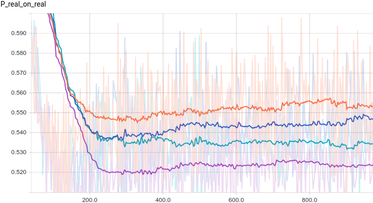
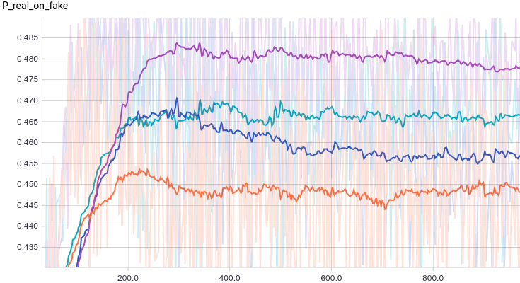
All four models quickly converge to a discriminator returning $1/2$ for all inputs. Because the problem is easy, there is not much of a difference between models. The following graphs show that the means and the standard deviations quickly converge to their true values:
 |
 |
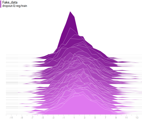
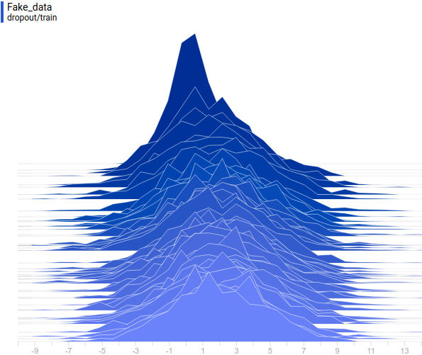
Below are distributions of real and generated examples during training. It can be seen that generated examples are almost indistinguishable from the real ones (though Tensorboard decided to choose different scales, so you have to look at the axis marks).
 |
 |
Let’s look at how the model was changing during training:
|
It can be seen that the discriminator is performing very well in the beginning of the training, but the generated distribution quickly “crawls” on top the the real one. In the end the generated has fitted the data so well that the discriminator becomes the $1/2$ constant and the solution converges.
Fitting a mixture of normal distributions I
Now let’s replace $p(x)=N(\mu,\sigma)$ with $p(x)=Mixture(N(\mu_1, \sigma_1), N(\mu_2, \sigma_2))$ so that the distribution of real data is bimodal. For this model we only need to change the code for generating real samples. Instead of returning a sample of a normally distributed random variable we return a sample from the mixture:
def data_batch(hparams):
  count = len(hparams.input_mean)
  componens = []
  for i in range(count):
      componens.append(
        tf.contrib.distributions.Normal(
          loc=hparams.input_mean[i],
          scale=hparams.input_stddev[i]))

  return tf.contrib.distributions.Mixture(
    cat=tf.contrib.distributions.Categorical(
      probs=[1./count] * count),
    components=componens)
      .sample(sample_shape=[hparams.batch_size, 1])
Below are the same graphs as in the previous experiment but for the bimodal distribution:
 |
 |
It is interesting to note that regularized models perform significantly better than non-regularized ones. However independently of the model it is easily seen that the generator can’t “fool” the discriminator now. Let’s see why is that.
 |
 |
Just like in the first experiment the generator approximates the data with a normal distribution. The reason for the approximation quality drop is that it’s impossible to approximate a bimodal distribution with a normal distribution which only has one mode. The modes are symmetric with respect to zero and it is easily seen from the graphs above that the data distribution is being approximated by all four models with a normal distribution with mean around zero and high standard deviation to cover variation from both modes. Let’s look at real and generated distributions to understand what’s going on:
 |
 |
Here’s the training process:
 |
This animation explains the case described above. The generator, not being powerful enough and only being able to approximate data with a bell curve, is stretching this curve too wide to span both modes. As a result the generator can only fool the discriminator in places where areas under generator density and real density curves are similar, i.e around the points where these curves intersect.
This however is not the only option. Let’s move the right mode a bit further to the right, so that the generator doesn’t capture it’s variance in the beginning of the training. Here is what we get:
 |
It can be seen that it’s most beneficial for the generator to approximate the left mode of the real data distribution. After this has happened, the generator starts trying to fit the right mode as well. This looks like oscillations of generator’s standard deviation in the second half of the animation. But all these attempts fail because the discriminator “locks” the generator by a high loss barrier which it can not break because of a too small learning rate. This effect is called mode collapsing.
Two examples above show two kinds of issues caused by a generator that is too simple for the problem. The first one is mode averaging, when the generator is trying to approximate multiple modes with just one and is bad everywhere as a result. The second one is mode collapsing when the generator only approximates a subset of all modes and is completely ignorant of other modes.
Both issues cause the discriminator to not converge to $1/2$, but also they cause a generative model to be worse. Mode averaging causes the generator to generate samples from between the modes with high probability, which is incorrect. Mode collapsing causes the generator to only generate samples from a subset of modes making it less reach than the original data distribution.
Fitting a mixture of normal distributions II
The reason for failing to “fool” the discriminator in the examples above was that the generator was too simple for the problem at hand. Let’s try to use a fully-connected neural network instead of a simple linear function:
def generator(self, input, hparams):
  # First fully connected layer with 256 features.
  input_size = 1
  features = 256
  weights = tf.get_variable(
    "weights_1", initializer=tf.truncated_normal(
      [input_size, features], stddev=0.1))
  biases = tf.get_variable(
    "biases_1", initializer=tf.constant(0.1, shape=[features]))
  hidden_layer = tf.nn.relu(tf.matmul(input, weights) + biases)

  # Second fully connected layer with 256 features.
  features = 256
  weights = tf.get_variable(
    "weights_2", initializer=tf.truncated_normal(
      [input_size, features], stddev=0.1))
  biases = tf.get_variable(
    "biases_2", initializer=tf.constant(0.1, shape=[features]))
  hidden_layer = tf.nn.relu(tf.matmul(input, weights) + biases)

  # Last linear layer for generating an example.
  output_size = 1
  weights = tf.get_variable(
    "weights_out", initializer=tf.truncated_normal(
      [features, output_size], stddev=0.1))
  biases = tf.get_variable(
    "biases_out",
     initializer=tf.constant(0.1, shape=[output_size]))
  return tf.matmul(hidden_layer, weights) + biases
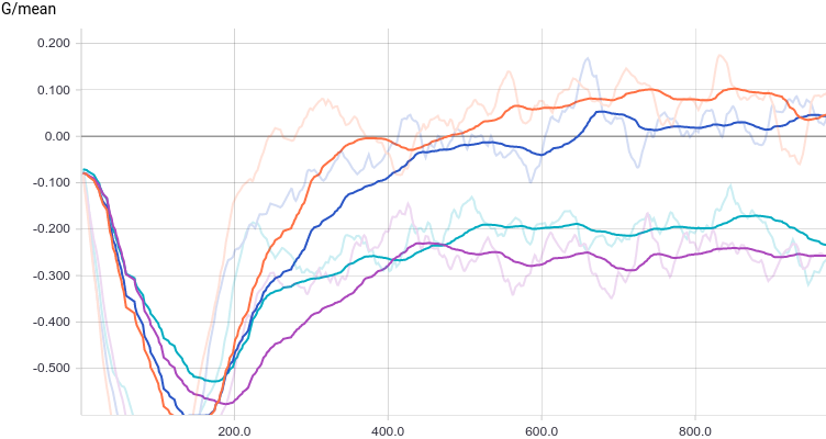
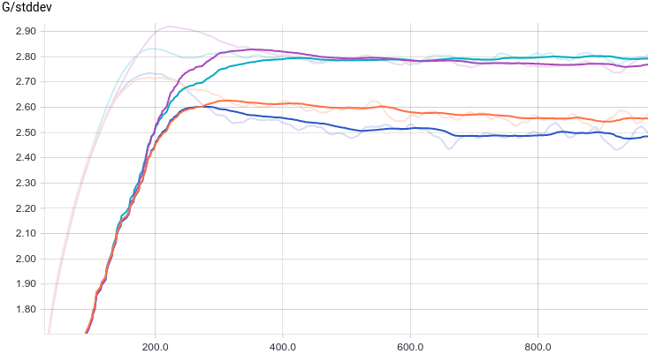
Let’s look at the training curves:
 |
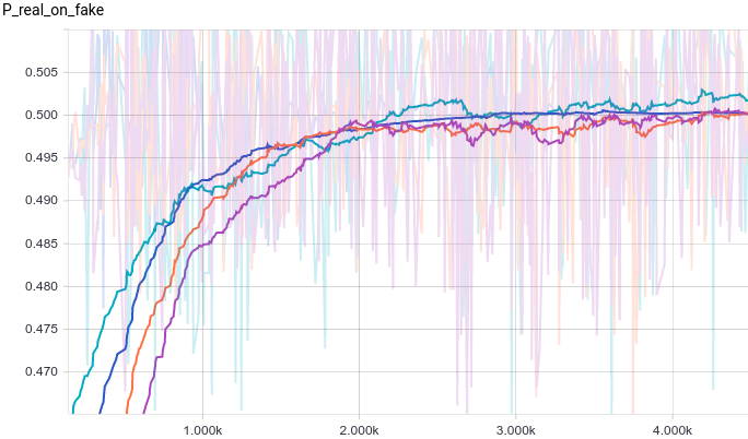 |
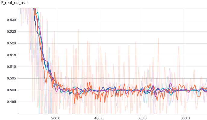
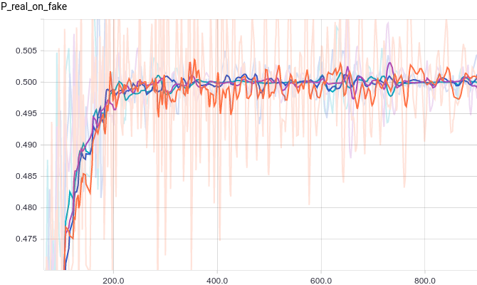
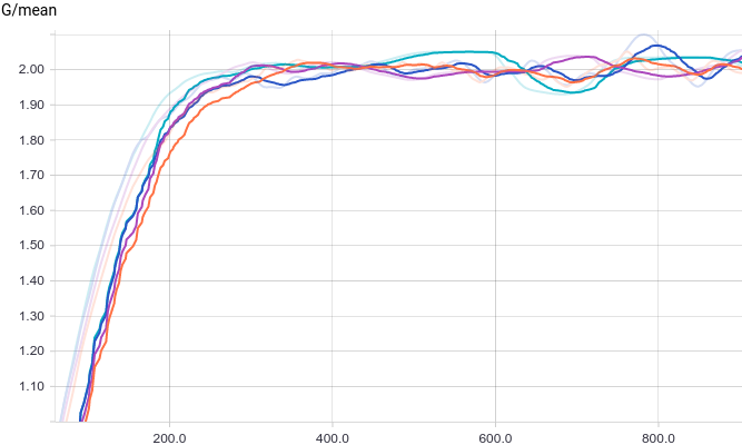
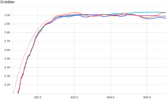
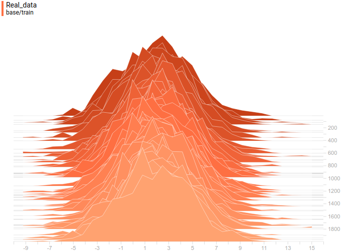
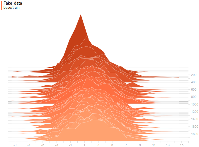
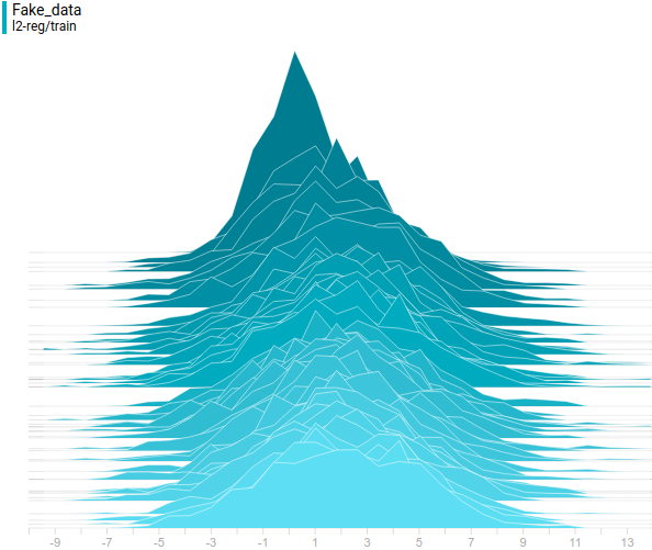
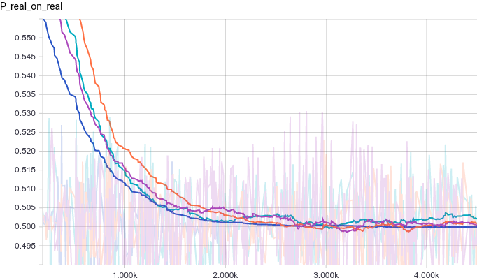
Because of the larger number of parameters the training is much noisier now. Discriminators in all models converge to something around $1/2$ but are quite unstable around it. Let’s look at the generator distribution:
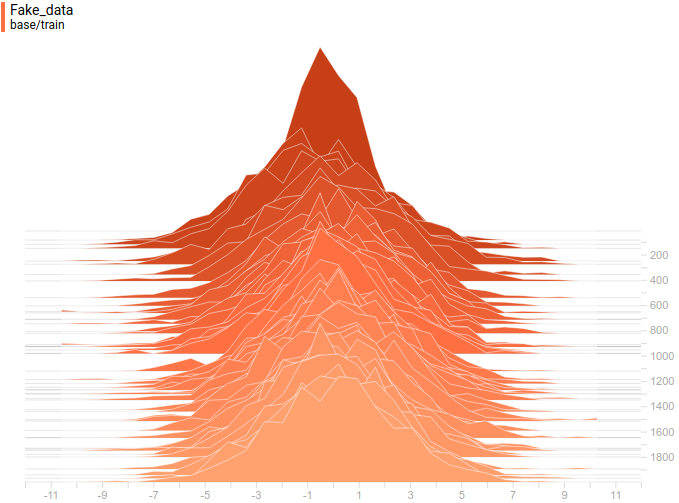
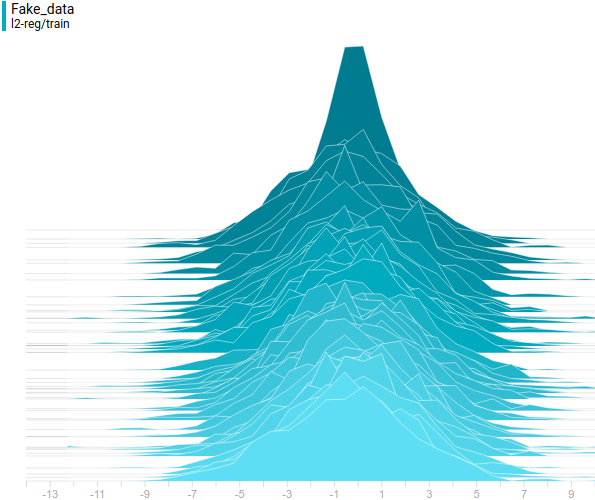
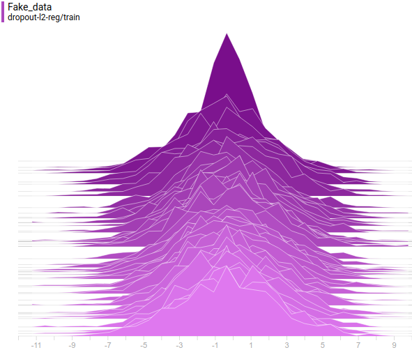
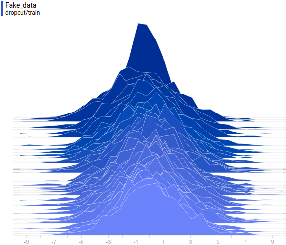
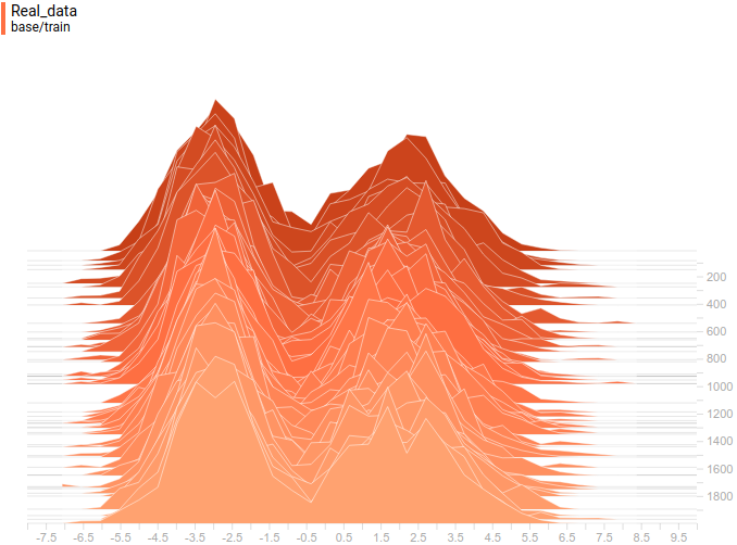 |
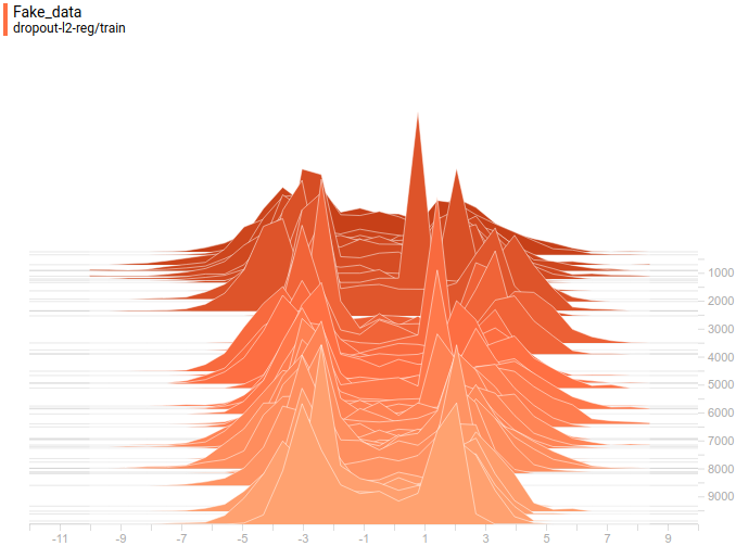 |
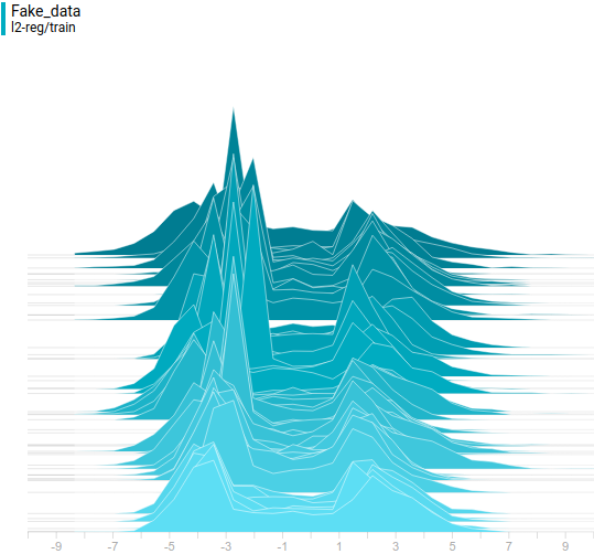
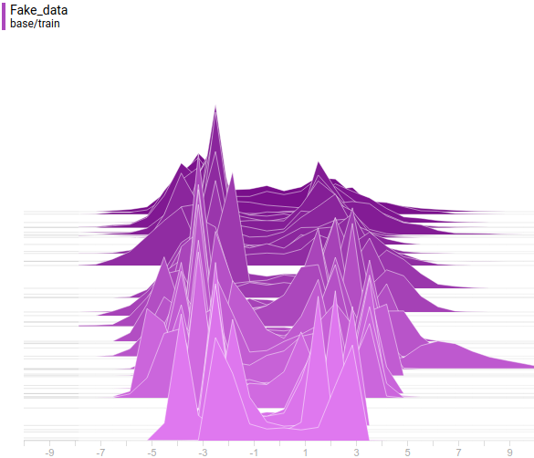
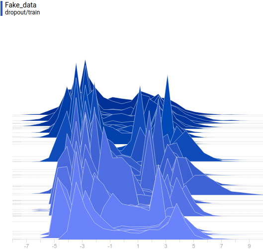
Generator distribution doesn’t exactly match the data distribution but it is quite close. The most regularized model is again the best performing one. It learned two modes that match the data distribution modes. The sizes of the learned distribution peaks are also similar to the ones in the data distribution. So, the neural-network based generator was able to learn a multimodal data distribution.
Here’s the training process:
 |
 |
These two animations show the training process of GANs on data distributions from the previous section. They show that using a sufficiently big generator with many parameters can approximate multimodal distributions, although quite crudely in our case. This confirms that the issues from the previous section are caused by the generator being too simple. Discriminators on these animations are significantly more noisy than in the fitting a normal distribution section, but nevertheless by the end of the training process they start looking like a noisy horizontal line $D(x)=1/2$.
Conclusion
GAN — is a model for approximating an arbitrary distribution by only sampling from that distribution. In this post we learned how this model works on a trivial example of fitting a normal distribution and on a more complex problem of fitting a bimodal distribution using a neural network. Both problems were solved with good accuracy which only required using a sufficiently complex generator model. In the next post we will move from simple test problems to real-world problems of generating samples from complex distributions of images.
Acknowledgements
Thanks Olga Talanova and Ruslan Login for reviewing this post. Thanks Ruslan Login for helping with images and animations. Thanks Andrei Tarashkevich for helping with converting it to Jekyll.