on
Probabilistic interpretaton of classical Machine Learning models
With this article I am starting a series covering generative models in machine learning. We will review classical machine learning (ML) problems, look at generative modelling, determine its differences from the classical ML problems, explore existing approaches, and dive into the details of the models based on deep neural networks. But before that we will look at probabilistic interpritations of classical Machine Learning problems as an introduction.
Classical machine learning problems
The two classical problems in machine learning are classification and regression. Let’s look closer at both problems, their setup, and simple examples with solutions.
Classification
Classification problem is a problem of assigning labels to objects. For example, if objects are represented by images, labels could reflect the content of the image: is there a pedestrian, is it a man or a woman, or what kind of dog is depicted. Usually, there is a list of mutually exclusive labels and a list of labeled objects for which these labels are known. The problem is to automatically label other objects using this data. Let’s formalize this definition. Assume there is a set of objects $X$, which can represent points on a plane, handwritten digits, pictures or musical compositions. Assume there also is a finite set of labels $Y$. These labels could be enumerated, e.g. in this case $Y=\{red, green, blue\}$ will be $Y=\{1, 2, 3\}$. If $Y=\{0, 1\}$, the problem is called “binary classification”; if there are more than two labels the problem is called just “classification” problem. In addition, there is a set $D=\{(x_i, y_i), x_i \in X, y_i \in Y, i=\overline{1,N}\}$ of labeled examples which will be used for learning and then automatic classification. Since we can’t know the class of an object for sure, we assume it to be a random variable. For simplicity we will also call it y. For example, an image of a dog can be classified as a dog with probability 99% and as a cat with probability 1%. This means that in order to classify any object we need to know the conditional distribution of the random variable given this object $p(y|x)$.
The problem of finding $p(y|x)$ given object $x$, a set of labels $Y$, and a set of labeled inputs $D=\{(x_i, y_i), x_i \in X, y_i \in Y,i=\overline{1,N}\}$ is called a classification problem.
Probabilistic interpretation of the classification problem
In order to solve this problem, we reformulate it in probabilistic framework. There is a set of objects $X$ and a set of labels $Y$. $\xi: \Omega \to X$ is a random variable representing an object from $X$. $\eta: \Omega \to Y$ is a random variable representing a label from $Y$. Consider a random variable $(\xi,\eta): \Omega \to (X, Y)$ with distribution $p(x, y)$, which represents the joint distribution of objects and their labels. This means that the labeled sample is exactly a sample from this distribution $(x_i, y_i) \sim p(x, y)$. We assume that all samples are independent and identically distributed (i.i.d.). The classification problem can now be reformulated as finding $p(y|x)$ given the sample $D=\{(x_i, y_i) \sim p(x, y), i=\overline{1,N}\}$.
Classification of two normally distributed variables
Let’s take a look and see how it all works on a simple example. Assume $X=R$, $Y=\{0, 1\}$, $p(x|y=0)=N(x; \mu_0,\sigma_0)$, $p(x|y=1)=N(x; \mu_1,\sigma_1)$, and $p(y=0)=p(y=1)=1/2$. This means that we have two gaussian curves from which we take samples with equal probabilities, and for any point in $R$ we need to classify from which gaussian this point was taken.
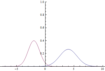 |
Since the domain of the gaussian is $R$, it is clear that these curves will intersect, meaning that there are points where probability densities $p(x|y=0)$ and $p(x|y=1)$ are equal.
Let’s find the conditional probability of labels:
\begin{equation} p(y|x)=\frac{p(x,y)}{p(x)}=\frac{p(x|y)p(y)}{\displaystyle\sum_{l \in Y}{p(x|l)p(l)}}=\{p(y)=\frac{1}{2}\}= \frac{p(x|y)}{\displaystyle\sum_{l \in Y}{p(x|l)}} \end{equation}
I.e. \begin{equation} p(y=i|x)=\frac{N(x;\mu_i, \sigma_i)}{\displaystyle\sum_{l \in Y}{N(x;\mu_l, \sigma_l)}} \end{equation}
Below is a chart with probability distribution $p(y=1|x)$:
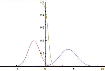 |
It can be seen, that close to the modes of the gaussians certainty of the model about the class is very high — probability is close to zero or to one. At the same time, when the curves intersect, the model can only randomly guess, which yields $p(x|y=1)=p(x|y=0)=1/2$.
Maximum likelihood method
Vast majority of the practical problems cannot be solved with the method above since $p(x|y)$ is usually not given explicitly. Instead we are given a set of labeled data $D=\{(x_i, y_i) \sim p(x, y), i=\overline{1,N}\}$ with unknown joint density distribution $p(x, y)$. In this case, the common approach is to use Maximum Likelihood Method (MLE). Formal definition and proofs can be found in your favourite Statistics textbook or using the link above. Here, I will describe the intuition behind the method.
Maximum likelihood method suggests, that if there is an unknown distribution $p(x)$ from which a set of samples $D=\{x_i \sim p(x), i=\overline{1,N}\}$, and some known parametric family of distributions $q(x|\theta)$, then in order to approximate $p(x)$, there is a need to find a vector of parameters which maximizes the likelihood of joint distribution $q(x_1,\dotsc, x_N|\theta)$, which is also called likelihood of the data. It is proved, that under reasonably generic conditions this is a consistent and unbiased estimator of the initial vector of parameters. If samples are taken from $p(x)$, i.e., the data is i.i.d., the joint distribution density is equivalent to the product of individual distributions densities:
\begin{equation} \arg\ \max_{\theta} q(x_1, \dotsc, x_N|\theta)=\arg\ \max_{\theta} \prod_{i=1..N} q(x_i|\theta) \end{equation}
Logarithm and non-negative constant multiplication are monotonic functions which do not change the extremums, so we take the logarithm of the joint density and multiply it by $\frac1N$:
\begin{equation} \arg\ \max_{\theta} \prod_{i=1..N} q(x_i|\theta)= \arg\ \max_{\theta} \frac{1}{N}\log\prod_{i=1..N} q(x_i|\theta)= \end{equation} \begin{equation} =\arg\ \max_{\theta} \frac{1}{N}\sum_{i=1..N} \log q(x_i|\theta) \end{equation}
The latter expression is in turn an unbiased and consistent estimator for the expected log likelihood:
\begin{equation} \arg\ \max_{\theta} \frac{1}{N}\sum_{i=1..N} \log q(x_i|\theta)= \arg\ \max_{\theta} \mathbb E_{x\sim p(x)} \log q(x|\theta) \end{equation}
This maximization problem can be rewritten as a minimization problem:
\begin{equation} \arg\ \max_{\theta} \mathbb E_{x\sim p(x)} \log q(x|\theta)= \arg\ \min_{\theta} \left( -\mathbb E_{x\sim p(x)} \log q(x|\theta) \right)= \arg\ \min_{\theta} H(p, q) \end{equation}
The latter term is called cross-entropy of the distributions $p$ and $q$. This is what is usually being optimized in supervised learning problems.
During this series of articles we will perform minimization with Stochastic Gradient Descent (SGD), specifically its extended model with adaptive moments. We will be using the fact that an average of gradients on a subsample (so called “mini-batch”) is an unbiased estimator of the gradient of the minimized function.
Classification of two normal distributions with logistic regression
Let’s try to solve the above problem with Maximum Likelihood method using a simple neural network $q(y|x, \theta)$. The resulting model is called logistic regression. Full code for the model can be found here. In this article we only cover the key points.
First, we need to generate data for our training. We need to create mini-batches of class labels and for each label generate a point from corresponding normal distribution:
def input_batch(dataset_params, batch_size):
    input_mean = tf.constant(dataset_params.input_mean, dtype=tf.float32)
    input_stddev = tf.constant(dataset_params.input_stddev,dtype=tf.float32)
    count = len(dataset_params.input_mean)
    labels = tf.contrib.distributions.Categorical(probs=[1./count] * count)
        .sample(sample_shape=[batch_size])
    components = []
    for i in range(batch_size):
        components
            .append(tf.contrib.distributions.Normal(
                loc=input_mean[labels[i]],
                scale=input_stddev[labels[i]])
            .sample(sample_shape=[1]))
    samples = tf.concat(components, 0)
    return labels, samples
Let’s define our classifier. It will be a simple neural network without hidden layers:
def discriminator(input):
    output_size = 1
    param1 = tf.get_variable(
        "weights",
        initializer=tf.truncated_normal([output_size], stddev=0.1)
    )
    param2 = tf.get_variable(
        "biases",
        initializer=tf.constant(0.1, shape=[output_size])
    )
    return input * param1 + param2
Also, let’s define a loss-function — cross-entropy between the distribution of real and predicted labels:
labels, samples = input_batch(dataset_params, training_params.batch_size)
predicted_labels = discriminator(samples)
loss = tf.reduce_mean(tf.nn.sigmoid_cross_entropy_with_logits(
    labels=tf.cast(labels, tf.float32),
    logits=predicted_labels)
)
Below are the training curves of two models: basic and with L2-regularization:
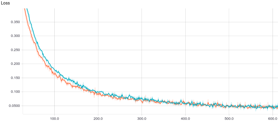 |
It can be seen, that both models converge quickly to a good result. The model without regularization showed better performance, since this problem does not require regularization, which can decrease learning speed. Let’s take a look at the training process:
 |
Observe, that the learned separating curve slowly converges to the analytical one. Also, the closer it gets to the analytical curve, the slower it converges due to the weaker loss function gradient.
Regression
Regression problem is a problem of predicting the values of one random variable $\eta: \Omega \to Y$ using the values of another vector random variable $\xi_i: \Omega \to X_i$. For example, predicting the height of a person using his or her gender and age. Similarly to the classification problem, there is a labeled sample $D=\{(x_i,y_i) \sim p(x, y), i=\overline{1,N}\}$. Precise prediction of the random variable is impossible, since it is random and is in fact a function so formally the problem is defined as predicting the conditional expectation:
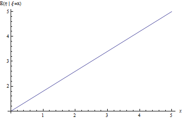
\[ f(x)=\mathbb E(\eta|\xi=x)= \int\limits_Y y\ p(y|x)\mathrm{d}y \]
Regression of linearly dependent variables with gaussian noise
Let’s take a look at the regression problem and see how it works on a simple example. Assume two independent random variables $\xi \sim Uniform(0, 10), \varepsilon \sim N(0,1)$. For example, the age of a tree and normal random noise. In this case we can assume that height of a tree is a random variable $\eta=a \xi + b + \varepsilon$. In this case, given linearity of the expectation and independency between $\xi$ and $\varepsilon$ we get:
\[ f(x)=E(\eta|\xi=x)= a\ E(\xi|\xi=x)+b+E(\varepsilon|\xi=x)= \] \[ =a\ E(\xi|\xi=x)+b+E(\varepsilon)= a\ x+b+0=a\ x+b \]
 |
Solving regression problem with Maximum Likelihood Estimation
Let’s formulate regression problem in MLE framework. Assume $q(y|x,\theta )=N(y; f(x; w), \sigma)$, where $w$ is a new vector of parameters. We need to find $f(x; w)$, the expectation of $q(y|x,\theta)$, so this is a correctly defined regression problem. This means:
\begin{equation} \arg\ \min_{\theta} H(p, q)= \arg\ \min_{\theta} \left( -\mathbb E_{x\sim p(x)} \log q(x|\theta) \right)= \end{equation} \begin{equation} =\arg\ \min_{\theta} \left( -\mathbb E_{x\sim p(x)} \log N\left(y;f\left(x,w\right),\sigma\right) \right)= \end{equation} \begin{equation} =\arg\ \min_{\theta} \left( -\mathbb E_{(x,y) \sim p(x, y)}\frac{\left(f\left(x; w\right) - y\right)^2}{\sigma^2} \right) \end{equation}
With sample average as consistent and unbiased estimator to the above:
\[ \arg\ \min_{\theta}\left( -\sum_{i=1..N}\frac{\left(f\left(x_i; w\right) - y_i\right)^2}{\sigma^2} \right) \]
This means that to solve this problem, it is convenient to minimize mean squared error on the training sample.
Regression of a variable with linear regression
Let’s solve the problem from the section above with MLE method using a simple neural network as the parametric family $q(y|x, \theta)$. This model is called linear regression. Full code can be found here. In this article we will cover the key points.
First, we need to generate data for training. We start with generating the input mini-batch $\xi \sim Uniform(0, 10), \varepsilon \sim N(0,1)$, after which we get a sample of initial variable $\eta=a \xi + b + \varepsilon$:
def input_batch(dataset_params, batch_size):
    samples = tf.random_uniform([batch_size], 0., 10.)
    noise = tf.random_normal([batch_size], mean=0., stddev=1.)
    labels = (dataset_params.input_param1 * samples + dataset_params.input_param2 + noise)
    return labels, samples
Let’s define our model. It will be a simple neural network without hidden layers:
def predicted_labels(input):
    output_size = 1
    param1 = tf.get_variable(
        "weights",
        initializer=tf.truncated_normal([output_size], stddev=0.1)
    )
    param2 = tf.get_variable(
        "biases",
        initializer=tf.constant(0.1, shape=[output_size])
    )
    return input * param1 + param2
Let’s also define the loss-function — the L2 distance between the distributions of actual and predicted values:
labels, samples = input_batch(dataset_params, training_params.batch_size)
predicted_labels = discriminator(samples)
loss = tf.reduce_mean(tf.nn.sigmoid_cross_entropy_with_logits(
    labels=tf.cast(labels, tf.float32),
    logits=predicted_labels)
)
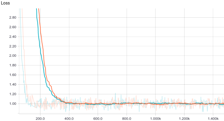
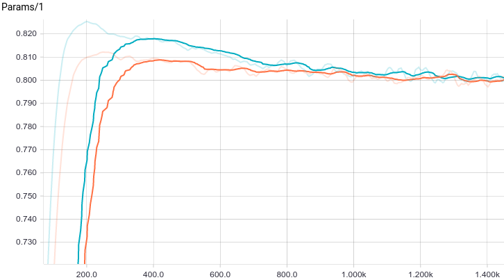
Below are the training curves of the models: basic and with L2-regularization (a.k.a ridge regression):
 |
 |
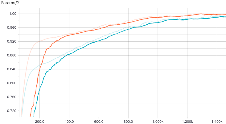 |
It can be seen, that both models converge quickly to a good result. The model without regularization showed better performance, since this problem does not require regularization, which can decrease the learning speed. Let’s take a look at the training process:
 |
It can be seen, that the learned expectation of $\eta$ consequently converges to the analytical one. Also, the close it gets to the analytical expectation, the slower it converges due to weaker loss function gradient.
Other problems
In addition to the described problems of classification and regression, there are other supervised learning problems, mostly related to correspondence between points and sequences: Object-to-Sequence, Sequence-to-Sequence, Sequence-to-Object. Also, there is a large variety of classical unsupervised learning problems: clusterization, missing data filling, and explicit or implicit fit of distribution, which is used for generative modelling. In our series, we will focus on the latter aspect.
Generative models
In the next chapter, we will take a look at generative models and see the differences between them and the classical discriminative models reviewed in this article. We will consider some simple examples of generative models and try to train a model for generating samples from a simple distribution.
Acknowledgements
Thanks Olga Talanova for reviewing this article and help translating it into English. Thanks Sofya Vorotnikova for comments, editing and proofreading the English version. Thanks Andrei Tarashkevich for helping convert this post into Jekyll.