Generative Modeling and AI

In the previous chapter we discussed classical discriminative models in machine learning and went over simple examples of such models. This time we are going to look at the bigger picture.

Artificial Intelligence

Artificial Intelligence (or AI) algorithms are able to solve problems typically solved by humans, ideally with matched or superior to human performance. It can be visual object recognition, understanding texts, controlling robots and performing logical or probabilistic inference. AI systems are algorithms that are able to decompose a fuzzy objective into these subproblems and effectively solve all of them. The general AI problem is not solved yet, but there are various approaches that might be the first steps towards solving it.

In the twentieth century, the most popular approach was based on the idea that the world can be described by a set of rules, such as physical laws. And even if all of them cannot be programmed directly, it is reasonable to assume that given a large enough number of these rules, an AI system will be able to efficiently exist and solve arbitrary problems in the world that they describe. Naive application of this approach does not take into account the stochastic nature of some naturally occurring phenomena. To account for that, the set of rules has to be converted into a probabilistic model for making stochastic decisions given random variables as inputs.

A complete description of the world would require so many rules that they could not be possibly programmed and supported manually. Hence, the idea to collect observations of the real world and use them to infer these rules automatically. This idea inherently supports both the natural stochasticity of some processes and the observed stochasticity that occurs when the causes of some deterministic processes are unknown. Automatic inference of the rules based on a set of observations is studied by the branch of mathematics called machine learning. Machine learning (or ML) is currently believed to be the most promising fundament for the general purpose AI.

Machine Learned AI

In the previous chapter we discussed classical problems of machine learning called classification and regression. We also implemented simple linear models for these problems called logistic and linear regressions. Real world problems are more complicated and have nonlinear nature. Models used for solving them are often based on artificial neural networks that usually outperform all other ML techniques on tasks with datasets that are large, have dense features and a lot of redundancy, such as analysing images, sounds, and texts.

These techniques are able to automatically infer rules from observations and are very successfully applied commercially. However, they have a flaw which makes them not powerful enough to be used for solving the AI problem: they are designed to solve a very specific problem, like distinguishing cat from dog images. It is obvious, that a model summarizing an image into a single number is losing a lot of data. One does not have to understand what a cat is to be able to find it in a picture, it is enough to detect its major features. Image classification task only requires finding specific objects, but not necessarily understanding the entire scene. Building a classifier for all possible combinations of objects and all possible logical connections between them is impossible in practice because of the exponential amount of observations needed and computation involved. Because of that, classical supervised learning is not a very good fit for AI. A different approach is needed.

Probabilistic formulation of the world understanding problem

So, we have a set of observations and need to somehow understand the process that generated these observations. Let’s formulate understanding using probabilistic language. Let each observation be an instance of a random variable $x: \Omega \to X$, $x \sim P(x)$. There is a set of these observations $D = {x_i \sim P(x), i=\overline{1,N}}$. Then “understanding” these observations can be thought of as recovering the distribution $P(x)$.

There are several approaches to solving this problem. One of the most generic methods is to introduce a latent variable. Suppose that every observation $x$ has a representation $z: \Omega \to Z$, $z \sim P(z)$. This representation can be thought of as a model’s “understanding” of the observation. For example the understanding of an image with a frame of a computer game would be the relevant internal state of the game and a camera position. Then $P(x) = \int_Z P(x|z)P(z)dz$. If one fix $P(z)$ to be a simple distribution and approximate $P(x|z)$ and $P(z|x)$ with neural networks, one can obtain $P(x)$ with standard deep learning methods and using the formula above. Then $P(x)$ can be used for probabilistic inference. More precise formulations of such models will be given in the following chapters but it is important to note that complicated models based on that idea require computing intractable integrals which is usually done by approximating them using MCMC or Variational Inference. Recovering $P(x)$ to draw samples from it is called a generative modelling problem.

There is an alternative idea. Having an explicit $P(x)$ is not strictly necessary, it can be obtained implicitly as well. If a model can “imagine” the world, it is safe to assume that the model understands it. For example, if one can draw a person in different poses and from different angles it implies understanding of human anatomy and laws of perspective. If a classifier (which can be a human) can’t distinguish an example generated by a model from a real observation then the model have understood how the process generating these observations works at least as good as that classifier or better. This idea inspired development of generative modelling with implicit $P(x)$ using models that, given a set of observations, are able to generalize them by implicitly capturing $P(x)$ and able to generate new sample observations, indistinguishable from real ones. Suppose $z \sim N(0, 1)$ or any other distribution that is easy to sample. Then, in very general conditions, there exists $f: Z \to X$ such that $f(z) \sim P(x)$. Instead of finding $P(x)$, $f(x)$ can be found and then samples from $P(x)$ can be generated as $f(z), z \sim N(0,1)$. $f(z)$ can’t be used in probabilistic inference directly, but inference is not always the goal. And even if it is, Monte-Carlo integration, that only requires samples, can often be enough. Generative Adversarial Networks model, which we will look into in the next chapter, belongs to this class of models.

Principal Component Analysis

Let’s look at a simple generative latent variable model. Let $x \sim P(x)$ be an observed random variable. For example it can be a height of a person or an image of an object. Suppose that this variable can be fully explained by a latent (not observed) variable $z \sim P(z)$. In this analogy $z$ could be a person’s age or an object’s class and orientation. Suppose that $z$ is normally distributed, i.e. $P(z) = N(z; 0, 1)$. Suppose now that the observed variable $x$ depends on $z$ linearly with a normally distributed noise, i.e. $P(x|z) = N(x; Wz + b, \sigma^2 I)$. This model is called Probabilistic Principal Component Analysis (PPCA) and it is basically a probabilistic interpretation of a classical Principal Component Analysis (PCA) model, where the observable $x$ depends on $z$ linearly without the noise.

Expectation Maximization

Expectation Maximization (EM) is an algorithm for training models with latent variables. The details can be found in specialized literature, but the general idea is quite simple:

1. Initialize the model with some initial values of parameters.
2. E-step. Fill in the latent variables with their expected values given current model parameters and observed variables.
3. M-step. Maximize likelihood of training data with fixed latent variables. For example, using gradient ascent on parameters.
4. Repeat (2, 3) while expected values of latent variables change significantly.

In M-step full convergence is not required. A single step of the gradient ascent is enough. In this case the algorithm is called Generalized EM (GEM).

Solving PCA with EM

Let’s apply EM and maximum likelihood to our PCA model to find optimal model parameters $\theta = (W, b, \sigma)$. Joint likelihood of the observed and latent variables can be expressed as:

\begin{equation} L(x|\theta)=\log P(x|\theta)=\log P(x|\theta) \int_z q(z)=\int_z q(z) \log P(x|\theta) \end{equation}

Where $q(z)$ is an arbitrary distribution. From here on conditioning on model parameters will be implied and we will not write it explicitly to make formulas easier to read.

\begin{equation} \int_z q(z) \log P(x|\theta)=\int_z q(z) \log \frac{P(x, z)}{P(z|x)}=\int_z q(z) \log \frac{P(x, z)q(z)}{q(z)P(z|x)}= \end{equation} \begin{equation} =\int_z q(z) \log P(x, z)-\int_z q(z) \log q(z)+\int_z q(z) \log \frac{q(z)}{P(z|x)}= \end{equation} \begin{equation} =\int_z q(z) \log P(x, z)+H\left(q\left(z\right)\right)+KL(q(z)||P(z|x)) \end{equation}

Where $KL(q(z)||P(z|x))=\int_z q(z) \log \frac{q(z)}{P(z|x)}$ is called $KL$-divergence between distributions $q(z)$ and $P(z|x)$. $H\left(q\left(z\right)\right)=-\int_z q(z) \log q(z)$ is called entropy of $q(z)$. $H\left(q\left(z\right)\right)$ does not depend on model parameters $\theta$, so this term can be ignored during optimization:

\begin{equation} L(x|\theta) \propto \int_z q(z) \log P(x, z)+KL(q(z)||P(z|x))= \end{equation} \begin{equation} =\int_z q(z) \log \left( P(x|z)P(z)\right)+KL(q(z)||P(z|x))= \end{equation} \begin{equation} =\int_z q(z) \log P(x|z)+\int_z q(z) \log P(z)+KL(q(z)||P(z|x)) \propto \end{equation} \begin{equation} \propto \int_z q(z) \log P(x|z)+KL(q(z)||P(z|x)). \end{equation}

$KL(q(z)||P(z|x))$ is non-negative and is equal to zero iff $q(z)=P(z|x)$. Keeping that in mind, let’s write down the EM-algorithm for this problem:

1. E: $q(z) := P(z|x)$. This will zero out the second term $KL(q(z)||P(z|x))$.
2. M: Maximize the first term $L(x|\theta) \propto \int_z q(z) \log P(x|z)$.

PPCA is a linear model, so it can be solved analytically. Instead of doing that we will try to solve it using generalized EM with one step of SGD on each M-step. Because the data is i.i.d., we get:

\begin{equation} L(x|\theta) \propto \int_z q(z) \log P(x|z)=\int_z q(z) \log \prod_{i=1}^{N} P(x_i|z_i)=\int_z q(z) \sum_{i=1}^{N} \log P(x_i|z_i) \end{equation}

Note that $\int_zq(z)f(z)$ is an expectation $E_{z \sim q(z)} f(z)$. Then

\begin{equation} \int_z q(z) \sum_{i=1}^{N} \log P(x_i|z_i)=E_{z \sim q(z)} \sum_{i=1}^{N} \log P(x_i|z_i) \propto E_{z \sim q(z)} \frac{1}{N}\sum_{i=1}^{N} \log P(x_i|z_i) \end{equation}

Because a single sample is an unbiased estimate of the expected value the next equation is approximately correct:

\begin{equation} E_{z \sim q(z)} \frac{1}{N}\sum_{i=1}^{N} \log P(x_i|z_i)=\frac{1}{N} \sum_{i=1}^{N} \log P(x_i|z_i). \end{equation}

Substituting $P(x|z) = N(x; Wz + b, \sigma^2 I)$ we get:

\begin{equation} L(x|\theta) \propto \frac{1}{N} \sum_{i=1}^{N} \log P(x_i|z_i)= \end{equation} \begin{equation} = \frac{1}{N} \sum_{i=1}^{N} \log\left(\frac{1}{\sqrt{\left(2 \pi \right)^d \left| \sigma^2 I\right|}} \exp\left(-\frac{||x_i - \left(Wz_i + b\right)||^2}{2 \sigma^2}\right)\right)= \end{equation} \begin{equation} = \frac{1}{N} \sum_{i=1}^{N} \log\left(\frac{1}{\sqrt{\left(2 \pi \sigma^2\right)^d}} \exp\left(-\frac{||x_i - \left(Wz_i + b\right)||^2}{2 \sigma^2}\right)\right)= \end{equation} \begin{equation} = \frac{1}{N} \sum_{i=1}^{N} \left( - \log \sqrt{\left(2 \pi \sigma^2\right)^d} - \frac{1}{2 \sigma^2}{||x_i - b - W z_i||}^2\right) \end{equation} or \begin{equation} L(x|\theta) \propto L^{*}(x|\theta)=-\frac{1}{N} \sum_{i=1}^{N} \left(d\log\left(\sigma^2\right) + \frac{1}{\sigma^2}{||x_i - b - W z_i||}^2\right) \end{equation}

Where $d$ is the dimensionality of the observed variable $x$. Now let’s rewrite the GEM-algorithm for PPCA. $P(x|z) = N(x; Wz + b, \sigma^2 I)$, so $P(z|x)=N\left(z; \left(W^T W + \sigma^2 I \right)^{−1} W^T\left(x − b\right), \sigma^2 \left(W^T W + \sigma^2 I \right)^{−1} \right)$. Then GEM-algorithm goes like so:

1. Initialize parameters $W, b, \sigma$ with sensible random initial values.
2. Sample ${x_i} \sim P(x)$. This basically means choosing a minibatch from the dataset.
3. Compute latent variables $z_i \sim P(z|x_i)$ or $z_i = \left(W^T W + \sigma^2 I \right)^{-1} W^T\left(x_i - b\right) + \varepsilon, \varepsilon \sim N(0, \sigma^2 \left(W^T W + \sigma^2 I \right)^{-1})$.
4. Substitute $x_i, z_i$ in formula (1) for $L^{*}(x|\theta)$ and do a single step of the gradient ascent on parameters $W, b, \sigma$. It is important to remember that $z_i$ is an input here and that the back propagation should not propagate inside them.
5. If both the data likelihood and expected values of latent variables do not change much, stop the training. Otherwise go to (2).

After the model is trained, generated observations can be obtained as samples from \begin{equation} P(x)=N(x; b, W W^T + \sigma^2 I) \end{equation}

Numerical solution for PCA

Let’s now train the PPCA model using standard SGD. To understand it better we will again examine how the model works on a toy example. The complete code can be found here and in this article only the key points will be highlighted.

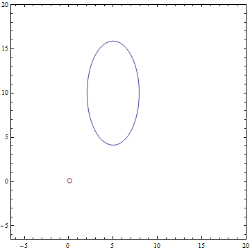
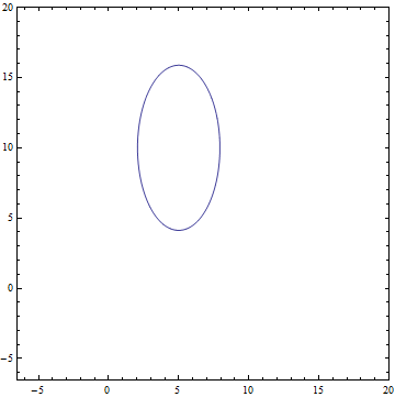
Let $P(x)=N(x;\begin{pmatrix} 5 \\ 10 \end{pmatrix}, \begin{pmatrix} 1.2^2 & 0 \\ 0 & 2.4^2 \end{pmatrix})$ — two-dimensional normal distribution with diagonal covariance matrix. $P(z)=N(z; 0, 1)$ — one-dimensional normal distributions of latent representations.

Fig. 1. Ellipse around the mean that covers 95% of points from $P(x)$.

The first thing to do is to generate the training data from $P(x)$:

def normal_samples(batch_size):
  def example():
    return tf.contrib.distributions.MultivariateNormalDiag(
     [5, 10], [1.2, 2.4]).sample(sample_shape=[1])[0]
  return tf.contrib.data.Dataset.from_tensors([0.])
    .repeat()
    .map(lambda x: example())
    .batch(batch_size)

Now let’s define model parameters:

input_size = 2
latent_space_size = 1
stddev = tf.get_variable(
  "stddev", initializer=tf.constant(0.1, shape=[1]))
biases = tf.get_variable(
  "biases", initializer=tf.constant(0.1, shape=[input_size]))
weights = tf.get_variable(
  "Weights",
   initializer=tf.truncated_normal(
     [input_size, latent_space_size], stddev=0.1))

Then latent representations can be obtained for the training data:

def get_latent(visible, latent_space_size, batch_size):
  matrix = tf.matrix_inverse(
    tf.matmul(weights, weights, transpose_a=True)
      + stddev**2 * tf.eye(latent_space_size))
  mean_matrix = tf.matmul(matrix, weights, transpose_b=True)
  # Multiply each vector in a batch by a matrix.
  expected_latent = batch_matmul(
    mean_matrix, visible - biases, batch_size)
  stddev_matrix = stddev**2 * matrix
  noise =
    tf.contrib.distributions.MultivariateNormalFullCovariance(
      tf.zeros(latent_space_size),
      stddev_matrix)
        .sample(sample_shape=[batch_size])
  return tf.stop_gradient(expected_latent + noise)

Note the tf.stop_gradient(...). This function prevents parameters inside the input subgraph to influence the gradient updates. This is needed so that $q(z) := P(z|x)$ would remain fixed during the M-step, which is required for EM to work correctly.

Let’s now define the loss function $L^{*}(x|\theta)$ to optimize on the M-step:

sample = dataset.get_next()
latent_sample = get_latent(sample, latent_space_size, batch_size)
norm_squared = tf.reduce_sum((sample - biases -
  batch_matmul(weights, latent_sample, batch_size))**2, axis=1)
loss = tf.reduce_mean(
  input_size * tf.log(stddev**2) + 1/stddev**2 * norm_squared)
train = tf.train.AdamOptimizer(learning_rate)
  .minimize(loss, var_list=[bias, weights, stddev], name="train")

Now the model is ready to be trained. Here is its training curve:

Fig. 2. PPCAs training curve.

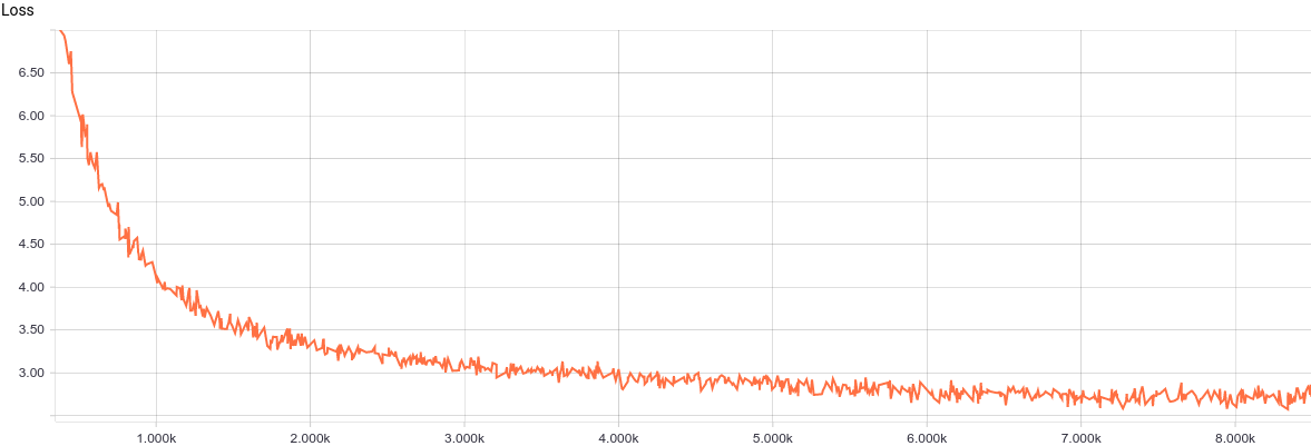It can be seen that the model converges quite smoothly and quickly because the problem is very simple. Here are the learned model parameters:

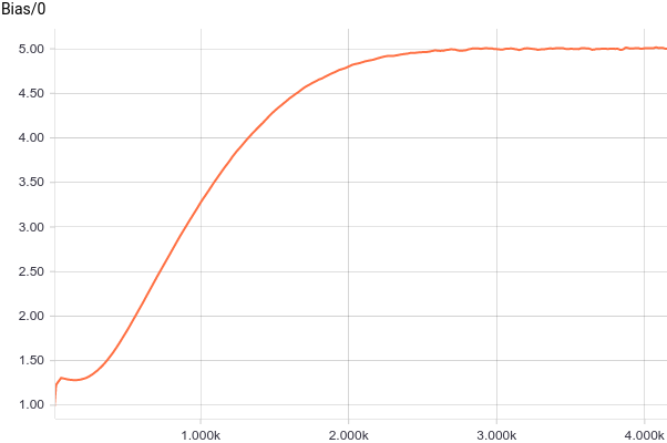
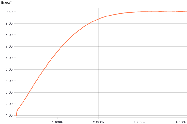
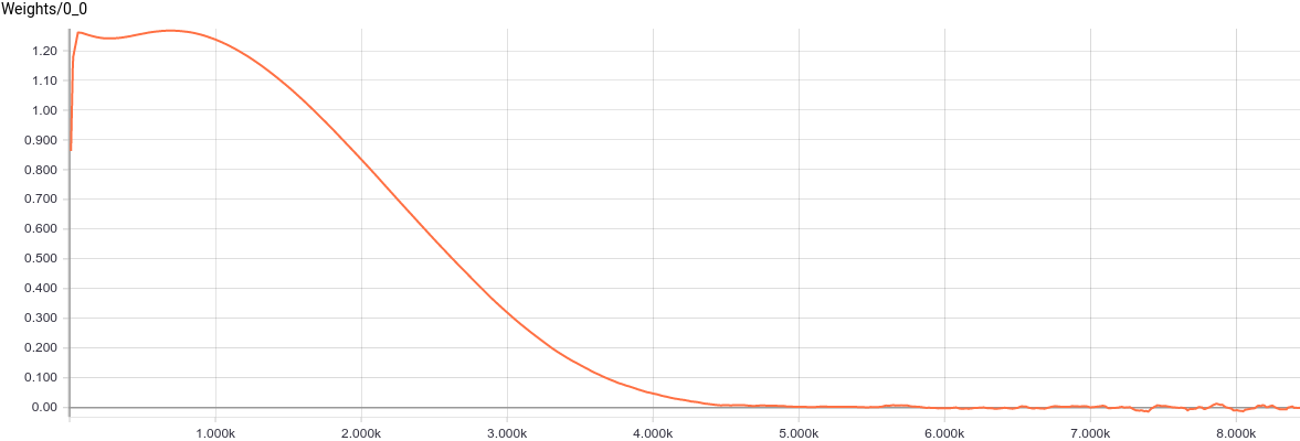
It can be seen that $b_i$ converge to analytical values $5$ and $10$ very quickly. Let’s now look at parameters $W, \sigma$:

Fig. 4. Learned parameter $\sigma$.

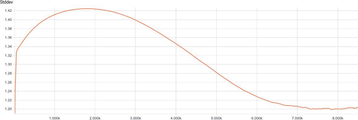It can be seen that $\sigma$ has converged to $1.2$, i.e. to the smallest variance axes of the input distribution, as expected.

Fig. 5. Learned parameters $W_{i0}$.

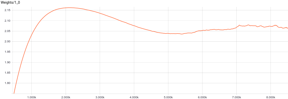$W$, in turn, has approximately converged to a value for which $W W^T + \sigma^2 I=\begin{pmatrix} 1.2^2 & 0 \\ 0 & 2.4^2 \end{pmatrix}$. Substituting these values in the model we get $$P(x)=N(x; b, W W^T + \sigma^2 I)=N(x; \begin{pmatrix} 5 \\ 10 \end{pmatrix}, \begin{pmatrix} 1.2^2 & 0 \\ 0 & 2.4^2 \end{pmatrix})$$, which means that we have recovered the data distribution.

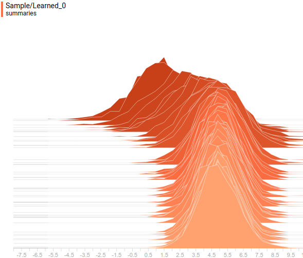
Let’s look at the data distributions. The latent variable is one-dimensional, so it is displayed as a one-dimensional distribution. The visible variable is two dimensional, but its true covariance matrix is diagonal so we will display it as two projections of the two-dimensional distribution on the coordinate axes. This is how projections of true and learned $P(x)$ on the first coordinate axis look like:

Fig. 6. The projection of the true $P(x)$ on the first coordinate axis.

Fig. 7. The projection of the learned $P(x|\theta)$ on the first coordinate axis.

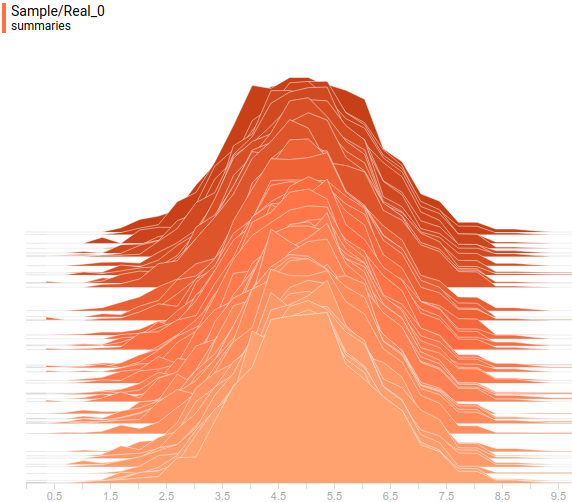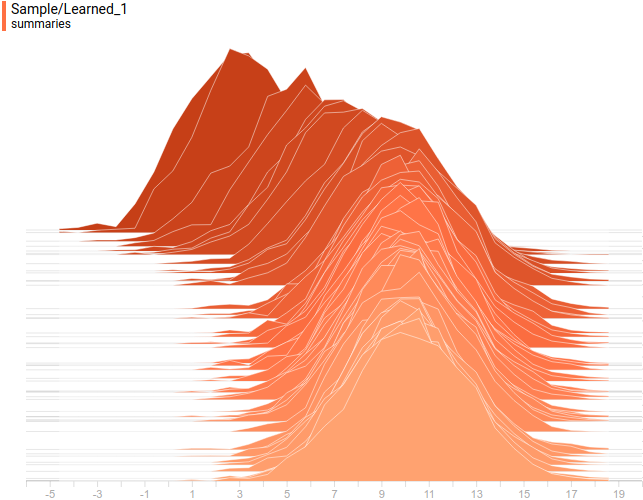
And this is how projections of true and learned $P(x)$ on the second coordinate axis look like:

Fig. 8. The projection of the true $P(x)$ on the second coordinate axis.

Fig. 9. The projection of the learned $P(x|\theta)$ on the second coordinate axis.

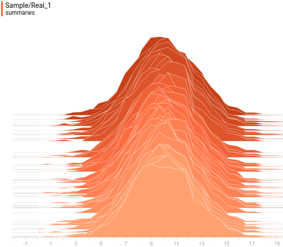This is how true and learned distributions $P(z)$ look like:

Fig. 10. True distribution $P(z)=N(z; 0, 1)$.

Fig. 11. Learned distribution $P(z|\theta)$.

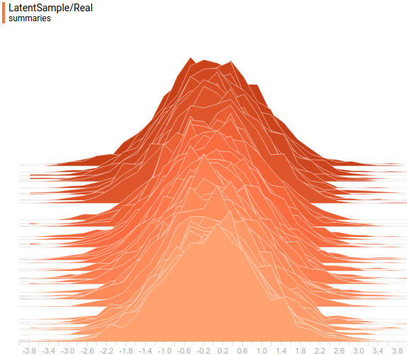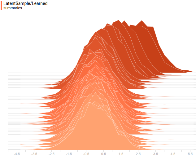It can be seen that all learned distributions have converged to distributions very similar to their true values. Let’s look at the training process for that model to be completely sure that it has actually recovered the true $P(x)$:

Fig. 12. The training process for the PPCA model. The learned $P(x|\theta)$ converges to the true $P(x)$.

Conclusion

The described model is a probabilistic version of the classical PCA model, which is a linear model. We reused the math for the EM algorithm from the original paper and built a numerical GEM algorithm on top of it. We showed that the resulting model converges to an analytical solution on a toy problem. Naturally if true $P(x)$ would not be normal the model would not recover it perfectly the same way that PCA can only perfectly fit data that forms a hyperplane in the feature space. To solve more complicated data distribution approximation problems more complicated nonlinear models are needed. One of these models called Generative Adversarial Networks will be described in the next chapter.

Acknowledgements

Thanks Olga Talanova for reviewing the text. Thanks Andrei Tarashkevich for helping with converting the text to Jekyll.